Fluid Dynamics Simulation in C++ and OpenGL

GitHub link: Here

After seeing the video “But How DO Fluid Simulators Work?” from the channel Inspecto, I thought it would be a simple effort to take the same core premise of a grid-based two-dimensional fluid simulator and extend it to include temperature. As it turns out, it was not a simple effort at all, but after a month of work on it and about a dozen headaches, I managed to get all the moving parts in place and generate a few nice gifs. This project was intended to be a learning experience to sharpen my C++ skills and get me acquainted to the basics of OpenGL, but since the programming side is heavy on the fundamentals, this breakdown will focus on the physics derivations used.

Full fluid, thermal, and blackbody simulation. Click through for high quality.

My starting point for the project was main reference for the Inspecto video, a white paper from the 2003 Game Developers Conference, “Real-Time Fluid Dynamics for Games” by Jos Stam. The paper describes the dynamics of a density scalar field $\rho$ and a velocity vector field $\mathbf{u}$ . The two fields are described by the following equations:

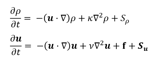
Both equations take a similar form. The first term on the right hand side describes advection, the motion of the fields through space due to the velocity field. The second term describes diffusion, with $\kappa$ representing the molecular diffusion constant for density, and $\nu$ representing the viscosity of the fluid. A source term describes external sources which we can create through user input. This leaves only $\mathbf{f}$ , the body forces on the fluid, which ended up being where most of the new math ended up going. More on that soon.

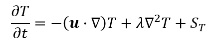
Simple fluid motion, without the effects of gravity or temperature. Click through for higher quality.

These two equations model the entirety of the physics of the original paper. To extend the behavior to include temperature effects, three steps were required: Adding a temperature field, adjusting temperature-dependent physical constants, and calculating body forces. The first step is simple enough, since the temperature field also follows an advection-diffusion equation:

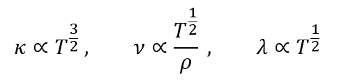
Temperature dependence is also straightforward. For an ideal gas, the constants follow the following polynomial relationships:

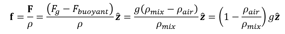
Buoyant forces ended up requiring a good amount of derivation, and a few assumptions to start out with. For a single fluid in empty space, the body force is simple: Everything accelerates downward at a constant rate of 9.8 meters per second. In order for buoyant forces to arise, the fluid must exist in a background medium, which I will just call “air”. The buoyant force on a single volume cell is derived from Bernoulli’s principle, as follows:

In order to move forward, we need to make a few assumptions:

The background medium has a fixed density $\rho_a^*$ , temperature $T_a$ , and molar mass $M_a$ . These are treated as set inputs to the simulator. Within the buoyancy equation we can assume the displaced air density is equal to $\rho_a^*$ .
The background medium and the fluid can both be modeled as an ideal gas with constant pressure. The pressure requirement is a bit shaky, but since I’ve been admonished that the fluid dynamical pressure field and the ideal gas pressure are “not the same” in a way that I haven’t found a good explanation for, we’re already playing fast and loose with the concept.
Each volume cell contains a constant number of particles. This describes a situation where the fluid under observation sorta “replaces” the background fluid, leading to the following values:

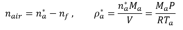
Armed with these assumptions and using some algebra, we can derive the density of the mixed fluid from the ideal gas law, and examine the value with the fluid is at the background temperature, $T_a$ :

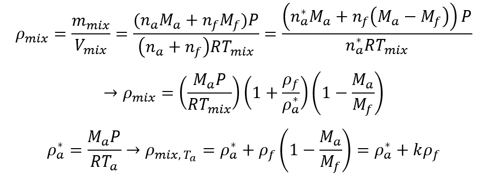
Here I’ve lumped the molar mass related term into a constant $k$ , for simplicity in interpreting these results. This seems to pass the sanity check, our mixed density is equal to the background density, adjusted by a factor determined by the relative molar masses. If the molar mass of the fluid is lower than that of the background, the mixed fluid is lighter than the air, and vice versa. The limits of our constant particle number assumption are glaring: If you add enough of a fluid which is lighter than air, eventually the mix weighs nothing at all, and then becomes negative. This corresponds to a case where all of the particles were replaced, and then some. It is jarring, but it is an edge case that never ended up causing problems in the simulator.

Plugging this back into the buoyancy equation:

This ends up being a nice simple formula, and it too passes a sanity check. When there is no fluid, the denominator goes to infinity, so the force goes to zero. That makes sense, since the background is completely uniform. As the fluid density increases, either a negative or a positive buoyant force is generated, depending on whether the fluid is lighter or heavier than air. That makes sense as well, less dense things rise.

Things are coming along smoothly, so let’s go ahead and vary that temperature away from $T_a$ , defining $T_f = T_a + \Delta T$ . Using the formula for the temperature of two mixed gases, and assuming that both gasses have the same specific heat (simply 3/2 for a monotonic ideal gas):

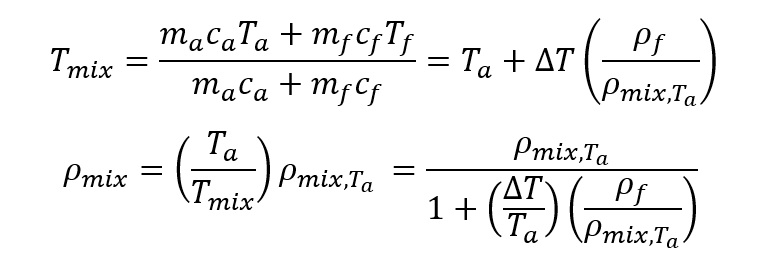
As always, sanity check time. At background temperature, we retrieve our previous result for the density. Good. When temperature goes up, $\Delta T$ becomes positive, and the density goes down. Similarly, a lower temperature increases the density. That checks out with what we know already, that hot gasses expand.

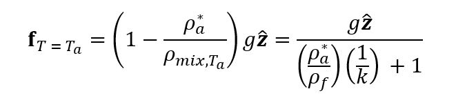
Finally, let’s plug all that in and find our completed buoyancy force:

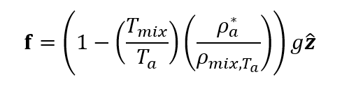
Now isn’t that beautifully simple? I would frame that and hang it up on my wall. The best part is that it tells us what we already know: Hot and light gasses rise, cold and dense gasses fall.

All of these pieces, together with a shader to describe blackbody radiation, come together to make the little gif of a flame you saw above. It’s a simple looking little thing, but I sure felt enormously proud once I finally saw it on screen.

Thanks for reading!

– Sean

Leave a Comment Cancel reply